Solutions to the exercises for the BBS course ‘Advanced group-sequential and adaptive confirmatory clinical trial designs, with R practicals using rpact’ on 13Sep2022
This R markdown file provides solutions to the exercises of the BBS course “Advanced group-sequential and adaptive confirmatory clinical trial designs, with R practicals using rpact”.
All materials related to this course are available on the BBS webpage at this link.
Load rpact
# Load rpactlibrary(rpact)
Installation qualification for rpact 4.2.0 has not yet been performed.
Please run testPackage() before using the package in GxP relevant environments.
packageVersion("rpact") # version should be version 3.0 or higher
[1] '4.2.0'
setLogLevel("DISABLED") # disable progress messages from e.g. getAnalysisResults # Also load tictoc for timing of the simulationslibrary(tictoc)
Exercise 1 (Group-sequential survival trial with efficacy and futility interim analyses)
Assume we plan a phase III, randomized, multicenter, open-label, two-arm trial with a time-to-event endpoint of OS. The general assumptions for the sample size assessment are:
2:1 randomization.
Uniform recruitment of 480 patients over 10 months (48 per month).
The dropout rate is 5% in both arms over 12 months.
The sample size section for OS states that the following additional assumptions were made:
Exponentially distributed OS in the control arm with a median of 12 months.
Median OS improvement vs. control of 4.9 months (medians 16.9 vs. 12 months, i.e. a HR of approximately 0.71).
Log-rank test at a two-sided significance level of 0.05, power 80%.
One interim analyses for efficacy (IA) and one final analysis using the O'Brien-Fleming boundaries approximated using the Lan-DeMets method. The first IA will be performed after 60% of information.
Exercise 1a (Sample size calculation)
Calculate the required number of events and timing of analysis for OS using the information fraction of 60%. Use the rpact functions getDesignGroupSequential and getSampleSizeSurvival.
Solution: We perform calculations at a one-sided significance level of 2.5% which gives the same sample size but is more compatible with the futility interim added in Part 1b.
# basic parametersinfofrac <-c(0.6, 1) # information fractionsalpha <-0.05/2# one-sidedbeta <-0.2accrualTime <-c(0, 10)accrualIntensity <-48# 48 pts over 10 monthsrandoratio <-2# 2:1 randomizationm2 <-12# median controlm1 <-16.9# median treatmentdo <-0.05# dropout same in both armsdoTime <-12# time at which dropout happensmaxn <- accrualIntensity * accrualTime[2]# Specify the group-sequential design design1 <-getDesignGroupSequential(sided =1, alpha = alpha, beta = beta,informationRates = infofrac, typeOfDesign ="asOF")# Calculate sample size for OS for this designsampleSizeOS1 <-getSampleSizeSurvival(design1,allocationRatioPlanned = randoratio, median2 = m2, median1 = m1, dropoutRate1 = do, dropoutRate2 = do, dropoutTime = doTime,accrualTime = accrualTime, accrualIntensity = accrualIntensity) # rpact summarysummary(sampleSizeOS1)
Sample size calculation for a survival endpoint
Sequential analysis with a maximum of 2 looks (group sequential design), one-sided overall significance level 2.5%, power 80%. The results were calculated for a two-sample logrank test, H0: hazard ratio = 1, H1: treatment median(1) = 16.9, control median(2) = 12, planned allocation ratio = 2, accrual time = 10, accrual intensity = 48, dropout rate(1) = 0.05, dropout rate(2) = 0.05, dropout time = 12.
Stage
1
2
Planned information rate
60%
100%
Cumulative alpha spent
0.0038
0.0250
Stage levels (one-sided)
0.0038
0.0238
Efficacy boundary (z-value scale)
2.669
1.981
Efficacy boundary (t)
0.658
0.786
Cumulative power
0.3123
0.8000
Number of subjects
480.0
480.0
Expected number of subjects under H1
480.0
Cumulative number of events
182.3
303.8
Expected number of events under H1
265.9
Analysis time
15.82
28.67
Expected study duration under H1
24.65
Exit probability for efficacy (under H0)
0.0038
Exit probability for efficacy (under H1)
0.3123
Legend:
(t): treatment effect scale
Exercise 1b (Addition of a futility interim analysis)
Now add an interim analysis for futility ONLY (i.e. no stopping for efficacy possible) after 30% of information where we stop the trial if the observed hazard ratio is above 1.
Hint: Use significance levels from design with efficacy only, add futility interim with minimal alpha-spending. The argument userAlphaSpending in getDesignGroupSequential helps.
Solution:
We spend a minimal alpha of 0.00001 at the futility interim analysis and use the alpha-spending from the O’Brien-Fleming-type alpha-spending function for the efficacy interim and the final analysis. In rpact, the futilityBounds are specified on the \(Z\)-scale and an observed hazard ratio 1 at the futility interim corresponds to a \(Z\)-score of 0. This leads to the following code:
# add the futility using the sig levels computed above and spending epsilon alpha at the futilitydesign2 <-getDesignGroupSequential(informationRates =c(0.3, infofrac),sided =1, alpha = alpha, beta = beta,typeOfDesign ="asUser", userAlphaSpending =c(0, design1$alphaSpent),futilityBounds =c(0, -Inf),bindingFutility =FALSE)# Calculate sample size for this designsampleSizeOS2 <-getSampleSizeSurvival(design2,allocationRatioPlanned = randoratio, median2 = m2, median1 = m1, dropoutRate1 = do, dropoutRate2 = do, dropoutTime = doTime,accrualTime = accrualTime, accrualIntensity = accrualIntensity) # rpact summarysummary(sampleSizeOS2)
Sample size calculation for a survival endpoint
Sequential analysis with a maximum of 3 looks (group sequential design), one-sided overall significance level 2.5%, power 80%. The results were calculated for a two-sample logrank test, H0: hazard ratio = 1, H1: treatment median(1) = 16.9, control median(2) = 12, planned allocation ratio = 2, accrual time = 10, accrual intensity = 48, dropout rate(1) = 0.05, dropout rate(2) = 0.05, dropout time = 12.
Stage
1
2
3
Planned information rate
30%
60%
100%
Cumulative alpha spent
0
0.0038
0.0250
Stage levels (one-sided)
0
0.0038
0.0238
Efficacy boundary (z-value scale)
Inf
2.669
1.981
Futility boundary (z-value scale)
0
-Inf
Efficacy boundary (t)
0
0.666
0.791
Futility boundary (t)
1.000
Cumulative power
0
0.3361
0.8000
Number of subjects
480.0
480.0
480.0
Expected number of subjects under H1
480.0
Cumulative number of events
96.9
193.7
322.9
Expected number of events under H1
266.8
Analysis time
10.12
16.72
31.74
Expected study duration under H1
25.48
Overall exit probability (under H0)
0.5000
0.0038
Overall exit probability (under H1)
0.0561
0.3361
Exit probability for efficacy (under H0)
0
0.0038
Exit probability for efficacy (under H1)
0
0.3361
Exit probability for futility (under H0)
0.5000
0
Exit probability for futility (under H1)
0.0561
0
Legend:
(t): treatment effect scale
We see that by adding the futility interim we increase the maximal number of events from 303.827705 to 322.8702626.
Exercise 1c (Power loss associated with the futility interim analysis)
How large is the power loss from adding this futility interim analysis, assuming we would not increase the number of events compared to the initial design above?
To compute the power loss of adding the futility, conservatively assuming it will be adhered to, i.e. we compute the power of the design with futility using the number of events of the design without futility.
Solution:
# power of design with futility at the number of events without futilitypower <-getPowerSurvival(design2, allocationRatioPlanned = randoratio, maxNumberOfEvents =ceiling(sampleSizeOS1$maxNumberOfEvents),median2 = m2, median1 = m1, dropoutRate1 = do, dropoutRate2 = do, dropoutTime = doTime,accrualTime = accrualTime, accrualIntensity = accrualIntensity,directionUpper =FALSE)# power, as compared to the specified 80%power$overallReject
[1] 0.7763167
So the power loss of adding the futility amounts to 0.0236833.
Bonus Exercise 1d (Timing of OS events)
How many OS events would be expected to occur until exactly 16 and 24 months, respectively, from first patient randomized?
Hint: getEventProbabilities.
Solution:
# Probability of an event until 16 months and 24 months probOS <-getEventProbabilities(time =c(16, 24), allocationRatioPlanned = randoratio, lambda2 =getLambdaByMedian(m2),lambda1 =getLambdaByMedian(m1),dropoutRate1 = do, dropoutRate2 = do, dropoutTime = doTime,accrualTime = accrualTime, accrualIntensity = accrualIntensity)probOS
Event probabilities at given time
User defined parameters
Time: 16.00, 24.00
Accrual time: 10.00
Accrual intensity: 48.0
lambda(1): 0.041
lambda(2): 0.0578
Planned allocation ratio: 2
Drop-out rate (1): 0.050
Drop-out rate (2): 0.050
Default parameters
kappa: 1
Drop-out time: 12.00
Time and output
Hazard ratio: 0.710
Maximum number of subjects: 480
Cumulative event probabilities: 0.3847, 0.5595
Event probabilities (1): 0.3506, 0.5193
Event probabilities (2): 0.4529, 0.6400
Legend
(i): values of treatment arm i
# Expected number of OS events
maxn * probOS$overallEventProbabilities
[1] 184.6677 268.5770
Expected number of events are 185 and 269 until months 16 and 24, respecticely.
Exercise 2 (Adaptive trial with a continuous endpoint)
A confirmatory, randomized and blinded study of an investigational drug against Placebo is planned in mild to moderate Alzheimer’s disease. The primary endpoint is the change from baseline in ADAS-Cog, a neuropsychological test battery measuring cognitive abilities, assessed 6 months after treatment initiation. The ADAS-Cog has a range of 0-70; we reverse its scale so that greater values are good. We consider our primary endpoint as approximately normally distributed, and for simplicity we assume a known standard deviation of 10. We believe that the improvement in the primary endpoint that can be achieved with the investigational drug is at least 4 points better than that under Placebo; and we want to have 80% chance of achieving a significant result if this is indeed the case. However, if the investigational drug is no better than Placebo, we want to have no more than 2.5% chance to claim success. This yields a sample size of approximately n=100 per treatment group for a trial with fixed sample size.
Exercise 2a (the “alpha calculus”)
We want to build in a “sanity check” mid-way through the trial. More precisely, we implement an interim analysis using the inverse normal method, with the following characteristics (all with respect to the primary endpoint):
Stop for futility if the investigational drug appears worse than Placebo
Stop for efficacy if the investigational drug appears “very significantly better” than Placebo (\(p < 0.0001\))
Which set of \((\alpha,\alpha_0,\alpha_1,\alpha_2)\) satisfies these conditions?
Hint: Use getDesignInverseNormal with a user-defined alpha-spending function and a binding futility boundary.
Solution:
The exercise specifies alpha=0.025, alpha0=0.5 (equivalent to a binding futility boundary at a \(Z\)-score of 0), and alpha1=0.0001. We compute alpha2 as follows.
d <-getDesignInverseNormal(typeOfDesign ="asUser", userAlphaSpending =c(0.0001,0.025), futilityBounds =0, bindingFutility =TRUE)d
Design parameters and output of inverse normal combination test design
User defined parameters
Type of design: User defined alpha spending
Futility bounds (binding): 0.000
Binding futility: TRUE
User defined alpha spending: 0.0001, 0.0250
Derived from user defined parameters
Maximum number of stages: 2
Stages: 1, 2
Information rates: 0.500, 1.000
Default parameters
Significance level: 0.0250
Type II error rate: 0.2000
Test: one-sided
Tolerance: 1e-08
Type of beta spending: none
Output
Cumulative alpha spending: 0.0001, 0.0250
Critical values: 3.719, 1.955
Stage levels (one-sided): 0.00010, 0.02531
This yields \(\alpha_2\) = d$stageLevels[2] = 0.0253.
What regulatory issues could this raise?
Solution The Regulator may not like that the final test is performed at a greater level (\(\alpha_2\)) than the overall level (\(\alpha\)). This is caused by cutting off a greater rejection region by the futility stop (right of \(\alpha_0\)) than adding to it by the efficacy stop (left of \(\alpha_1\)), and by compensating for this imbalance through a higher conditional error function (\(\alpha_2 > \alpha\); so-called “buy-back alpha” from the futility stop).
Exercise 2b (early stopping and sample size adaptation)
At the interim analysis after \(n_1\) = 50 patients per group, we observe an average ADAS-Cog improvement of 4 points under the investigational drug and of 1 point under Placebo. Should we stop or continue the trial?
Hint: getDataset to define the input dataset and getAnalysisResults to analyse it.
Solution
We should continue the trial, since our drug is neither worse nor very significantly better than Placebo:
Sequential analysis with 2 looks (inverse normal combination test design), one-sided overall significance level 2.5%. The results were calculated using a two-sample t-test, normal approximation test, equal variances option. H0: mu(1) - mu(2) = 0 against H1: mu(1) - mu(2) > 0. The conditional power calculation with planned sample size is based on overall effect = 3 and overall standard deviation = 10.
Stage
1
2
Fixed weight
0.707
0.707
Cumulative alpha spent
<0.0001
0.0250
Stage levels (one-sided)
<0.0001
0.0253
Efficacy boundary (z-value scale)
3.719
1.955
Futility boundary (z-value scale)
0
Cumulative effect size
3.000
Cumulative (pooled) standard deviation
10.000
Stage-wise test statistic
1.500
Stage-wise p-value
0.0668
Inverse normal combination
1.500
Test action
continue
Conditional rejection probability
0.1030
Planned sample size
100
Conditional power
0.5931
95% repeated confidence interval
[-4.438; 10.438]
Repeated p-value
\(\rightarrow\)\(p_1=0.0668\), and \(\alpha_1=0.0001<0.0668<0.5=\alpha_0\).
At the same time, there is a change in strategy, and we now want 90% power at an improvement of 4 points over placebo. Determine the sample size per treatment group for the second stage of the trial, in light of the interim results.
Hint: Calculate second stage sample size using getSampleSizeMeans with type I error equal to the conditional rejection probability from the previous part.
Solution
We compute the sample size necessary for 90% conditional power; we round up and check:
getSampleSizeMeans(alpha=result1$conditionalRejectionProbabilities[1], beta =0.1, alternative =4, stDev =10, normalApproximation =TRUE)$nFixed
Sequential analysis with 2 looks (inverse normal combination test design), one-sided overall significance level 2.5%. The results were calculated using a two-sample t-test, normal approximation test, equal variances option. H0: mu(1) - mu(2) = 0 against H1: mu(1) - mu(2) > 0. The conditional power calculation with planned sample size is based on assumed effect = 4 and assumed standard deviation = 10.
Stage
1
2
Fixed weight
0.707
0.707
Cumulative alpha spent
<0.0001
0.0250
Stage levels (one-sided)
<0.0001
0.0253
Efficacy boundary (z-value scale)
3.719
1.955
Futility boundary (z-value scale)
0
Cumulative effect size
3.000
Cumulative (pooled) standard deviation
10.000
Stage-wise test statistic
1.500
Stage-wise p-value
0.0668
Inverse normal combination
1.500
Test action
continue
Conditional rejection probability
0.1030
Planned sample size
164
Conditional power
0.9027
95% repeated confidence interval
[-4.438; 10.438]
Repeated p-value
\(\rightarrow\)\(n_2=82\) per treatment group
Exercise 2c (final inference)
In the second stage of the trial, we observe an average ADAS-Cog improvement of only 3 points under the investigational drug and of 1 point under Placebo.
Can we reject the null hypothesis and claim superiority of the investigational drug over placebo?
Solution
Using the inverse normal method as planned, we can reject the null hypothesis and claim superiority of the investigational drug over placebo. More precisely, the combination test statistic after the second stage is 1.966, exceeding the critical value \(u_{0.0253}=1.955\) (where \(u_\alpha\) is the \((1-\alpha)\)-quantile of \(N(0,1)\)). Note that we test at the local level \(\alpha_2=0.0253\).
Sequential analysis with 2 looks (inverse normal combination test design), one-sided overall significance level 2.5%. The results were calculated using a two-sample t-test, normal approximation test, equal variances option. H0: mu(1) - mu(2) = 0 against H1: mu(1) - mu(2) > 0.
Stage
1
2
Fixed weight
0.707
0.707
Cumulative alpha spent
<0.0001
0.0250
Stage levels (one-sided)
<0.0001
0.0253
Efficacy boundary (z-value scale)
3.719
1.955
Futility boundary (z-value scale)
0
Cumulative effect size
3.000
2.379
Cumulative (pooled) standard deviation
10.000
9.968
Stage-wise test statistic
1.500
1.281
Stage-wise p-value
0.0668
0.1002
Inverse normal combination
1.500
1.966
Test action
continue
reject
Conditional rejection probability
0.1030
95% repeated confidence interval
[-4.438; 10.438]
[0.014; 4.863]
Repeated p-value
Final p-value
0.0243
Final confidence interval
[0.014; 4.933]
Median unbiased estimate
2.450
Compute the overall (“exact”) p-value and confidence interval for the adaptive trial.
Solution
From the commands above we also obtain: \(p=0.02435; \; CI=(0.014,4.93)\)
What would a “naive” z-test have concluded, based on all observations and ignoring the adaptive nature of the trial? What is your interpretation of the situation?
Solution
A “naive” z-test would not have been able to reject the null hypothesis:
Sequential analysis with 2 looks (group sequential design), one-sided overall significance level 2.5%. The results were calculated using a two-sample t-test, normal approximation test, equal variances option. H0: mu(1) - mu(2) = 0 against H1: mu(1) - mu(2) > 0.
Stage
1
2
Planned information rate
50%
100%
Cumulative alpha spent
<0.0001
0.0250
Stage levels (one-sided)
<0.0001
0.0253
Efficacy boundary (z-value scale)
3.719
1.955
Futility boundary (z-value scale)
0
Cumulative effect size
3.000
2.379
Cumulative (pooled) standard deviation
10.000
10.000
Overall test statistic
1.500
1.933
Overall p-value
0.0668
0.0266
Test action
continue
accept
Conditional rejection probability
0.1030
95% repeated confidence interval
[-4.438; 10.438]
[-0.027; 4.785]
Repeated p-value
Final p-value
0.0263
Final confidence interval
[-0.027; 4.816]
Median unbiased estimate
2.390
Note that the definition of dat3 with the “cumulative” commands is necessary because otherwise always a “global” variance (accounting for the mean difference in the stages) is calculated.
Here we ignore the adaptive nature of the trial: we lump all data together (ignoring the sample size adaptation), and we test at the nominal level \(\alpha =0.025\) (ignoring the possibility of early stopping). The second stage of the trial, showing less of a treatment effect, carries greater weight in this “naive” (that is, incorrect) version of the test. Note that it can go both ways: in other examples, the adaptive (correct) version of the test may be the one that fails to reject the null hypothesis. In less borderline situations, both tests will lead to the same conclusion. Proposals have been made in the literature for dealing with borderline situations.
Exercise 3 (Sample size calculation for testing proportions)
Suppose a trial should be conducted in 3 stages where at the first stage 50%, at the second stage 75%, and at the final stage 100% of the information should be observed. O’Brien-Fleming boundaries should be used with one-sided \(\alpha = 0.025\) and non-binding futility bounds 0 and 0.5 for the first and the second stage, respectively, on the z-value scale.
The endpoints are binary (failure rates) and should be compared in a parallel group design, i.e., the null hypothesis to be tested is \(H_0:\pi_1 - \pi_2 = 0\,,\) which is tested against the alternative \(H_1: \pi_1 - \pi_2 < 0\,.\)
Exercise 3a (sample size calculation)
What is the necessary sample size to achieve 90% power if the failure rates are assumed to be \(\pi_1 = 0.40\) and \(\pi_2 = 0.60\)? What is the optimum allocation ratio?
Solution
The summary command provides a table for the study design parameters:
Sequential analysis with a maximum of 3 looks (group sequential design), one-sided overall significance level 2.5%, power 90%. The results were calculated for a two-sample test for rates (normal approximation), H0: pi(1) - pi(2) = 0, H1: pi(1) = 0.4, control rate pi(2) = 0.6.
Stage
1
2
3
Planned information rate
50%
75%
100%
Cumulative alpha spent
0.0021
0.0105
0.0250
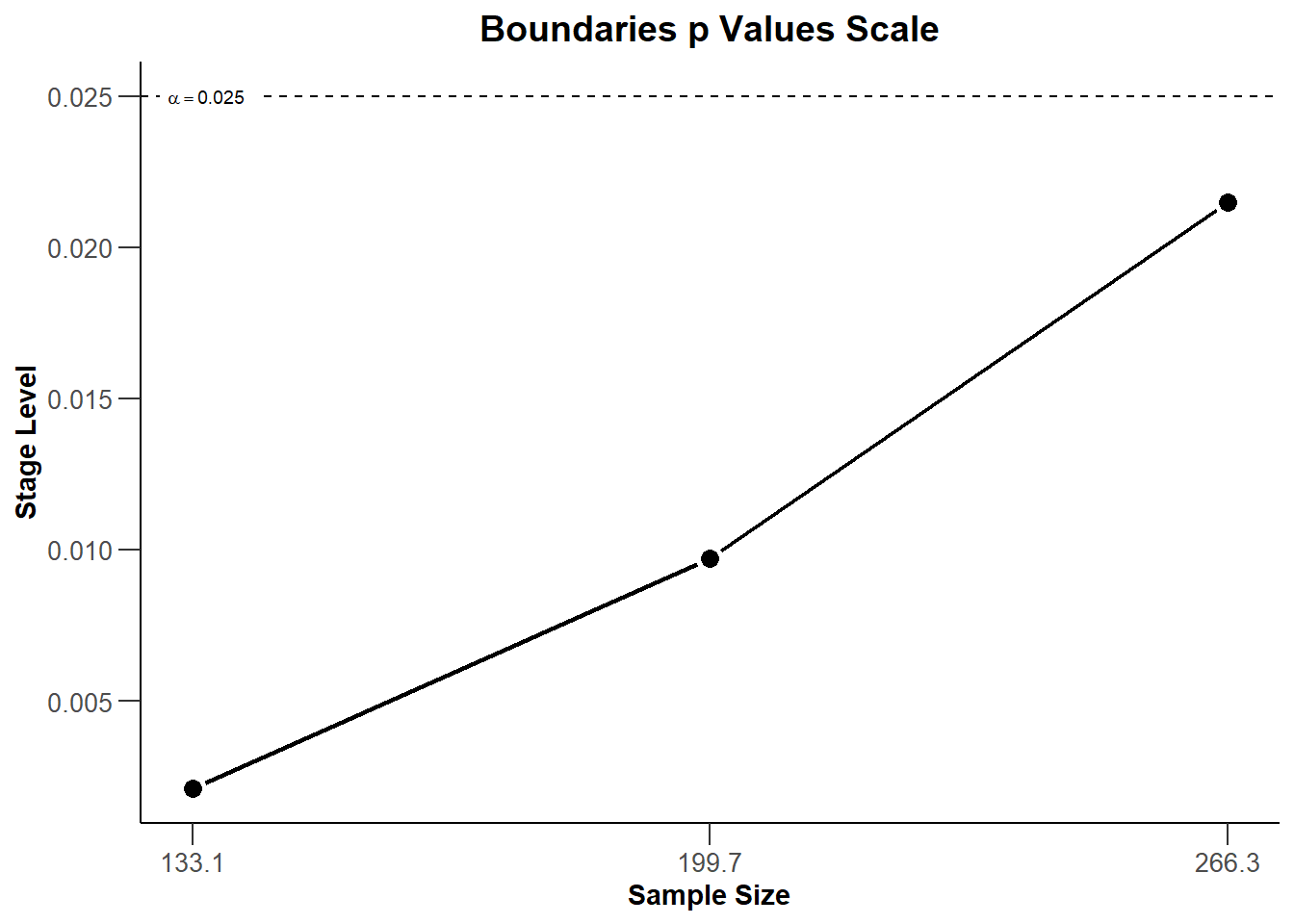
Stage levels (one-sided)
0.0021
0.0097
0.0215
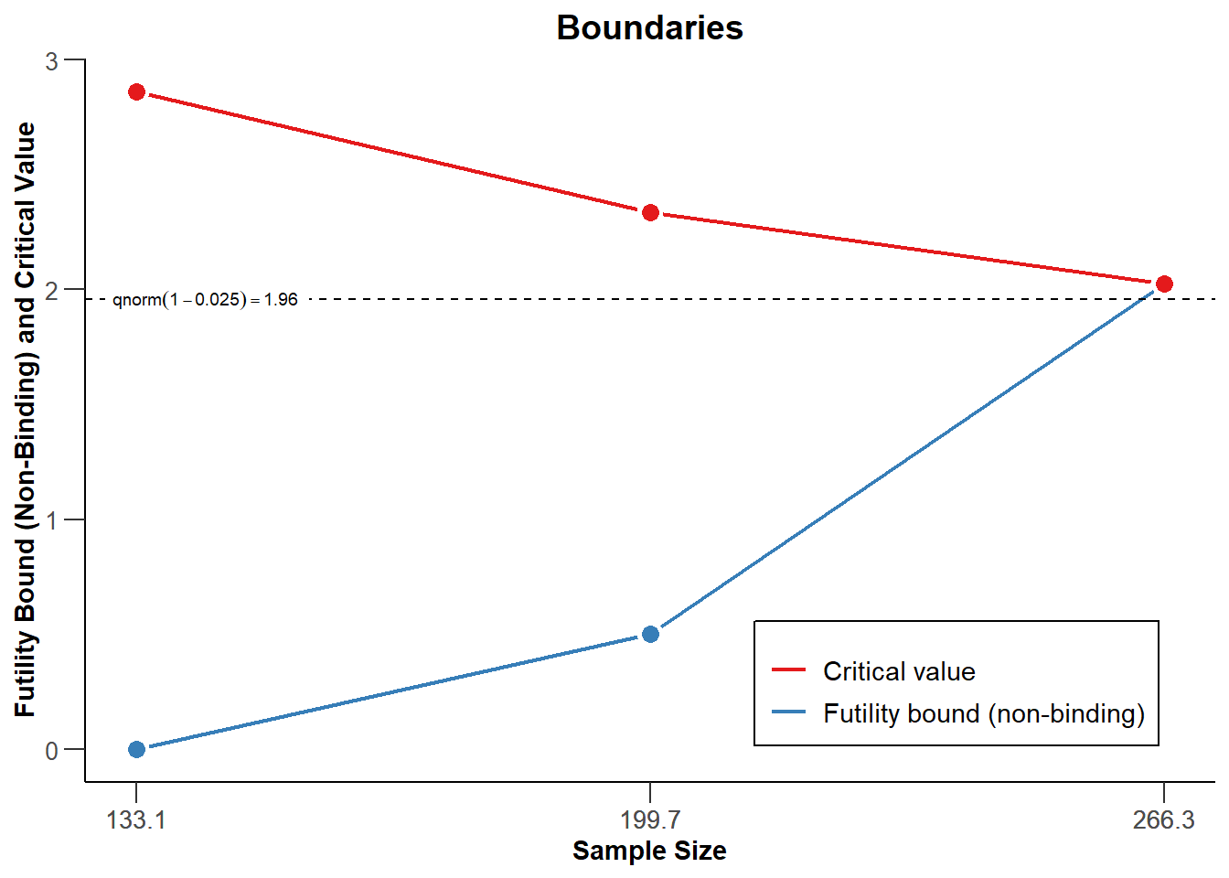
Efficacy boundary (z-value scale)
2.863
2.337
2.024
Futility boundary (z-value scale)
0
0.500
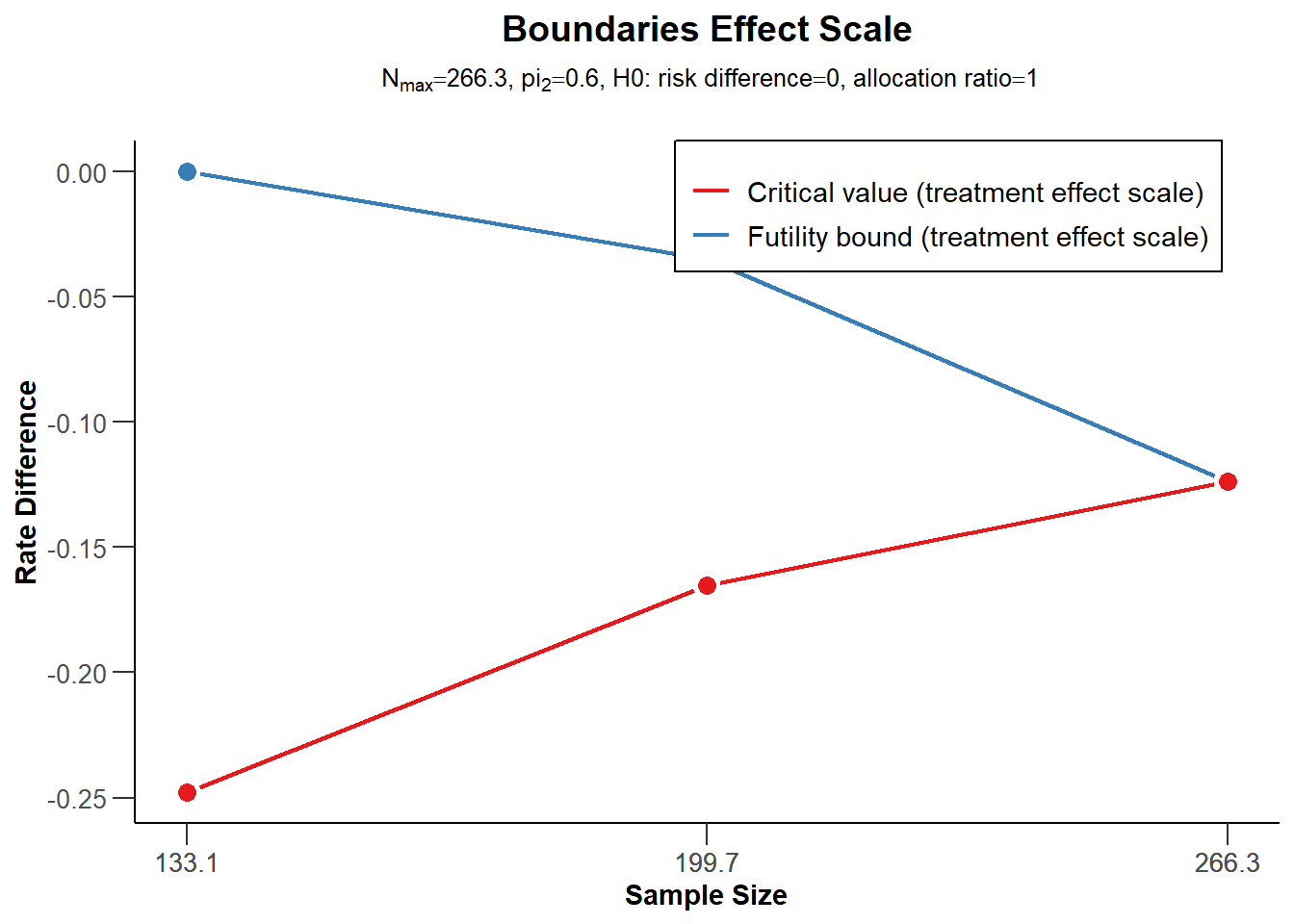
Efficacy boundary (t)
-0.248
-0.165
-0.124
Futility boundary (t)
0.000
-0.035
Cumulative power
0.2958
0.6998
0.9000
Number of subjects
133.1
199.7
266.3
Expected number of subjects under H1
198.3
Overall exit probability (under H0)
0.5021
0.2275
Overall exit probability (under H1)
0.3058
0.4095
Exit probability for efficacy (under H0)
0.0021
0.0083
Exit probability for efficacy (under H1)
0.2958
0.4040
Exit probability for futility (under H0)
0.5000
0.2191
Exit probability for futility (under H1)
0.0100
0.0056
Legend:
(t): treatment effect scale
The optimum allocation ratio is 1 in this case but calculated numerically, therefore slightly unequal 1:
r <-getSampleSizeRates(dGS, pi1 =0.4, pi2 =0.6, allocationRatioPlanned =0)r$allocationRatioPlanned
[1] 0.9999976
round(r$allocationRatioPlanned,5)
[1] 1
Exercise 3b (boundary plots)
Illustrate the decision boundaries on different scales.
Solution
plot(r, type =1)
plot(r, type =2)
plot(r, type =3)
Exercise 3c (power assessment)
Suppose that \(N = 280\) subjects were planned for the study. What is the power if the failure rate in the active treatment group is \(\pi_1 = 0.50\)?
Solution
The power is much reduced as compared to the case pi1 = 0.4 (where it exceeds 90%):
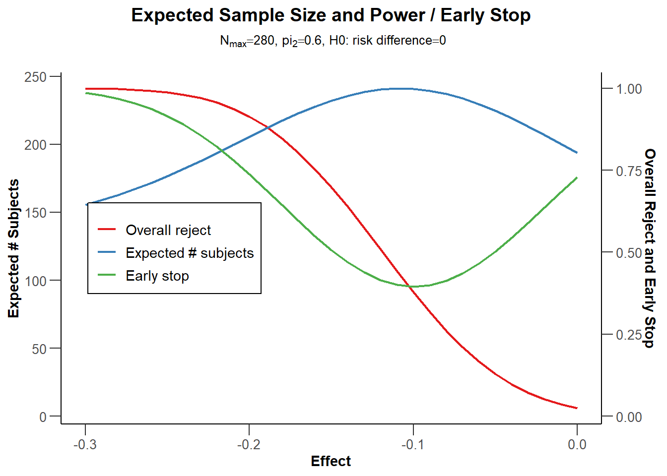
Illustrate power, expected sample size, and early/futility stop for a range of alternative values.
Solution
Specifying pi1 = c(0.3,0.6) provides a range of power and ANS values:
power <-getPowerRates(dGS, maxNumberOfSubjects =280, pi1 =c(0.3,0.6), pi2 =0.6,directionUpper =FALSE)plot(power, type =6)
Exercise 4 (Sample size reassessment for testing proportions)
Using an adaptive design, the sample size from Example 3 in the last interim can be increased up to a 4-fold of the originally planned sample size for the last stage. Conditional power 90% based on the observed effect sizes (failure rates) is used to increase the sample size.
Exercise 4a (assess power)
Use the inverse normal method to allow for the sample size increase and compare the test characteristics with the group sequential design from Example 3.
Solution
Define the inverse normal design and perform two simulations, one without and one with SSR:
Note that the sample sizes will be calculated under the assumption that the conditional power for the subsequent stage is 90%. If the resulting sample size is larger, the upper bound (4*70 = 280) is used.
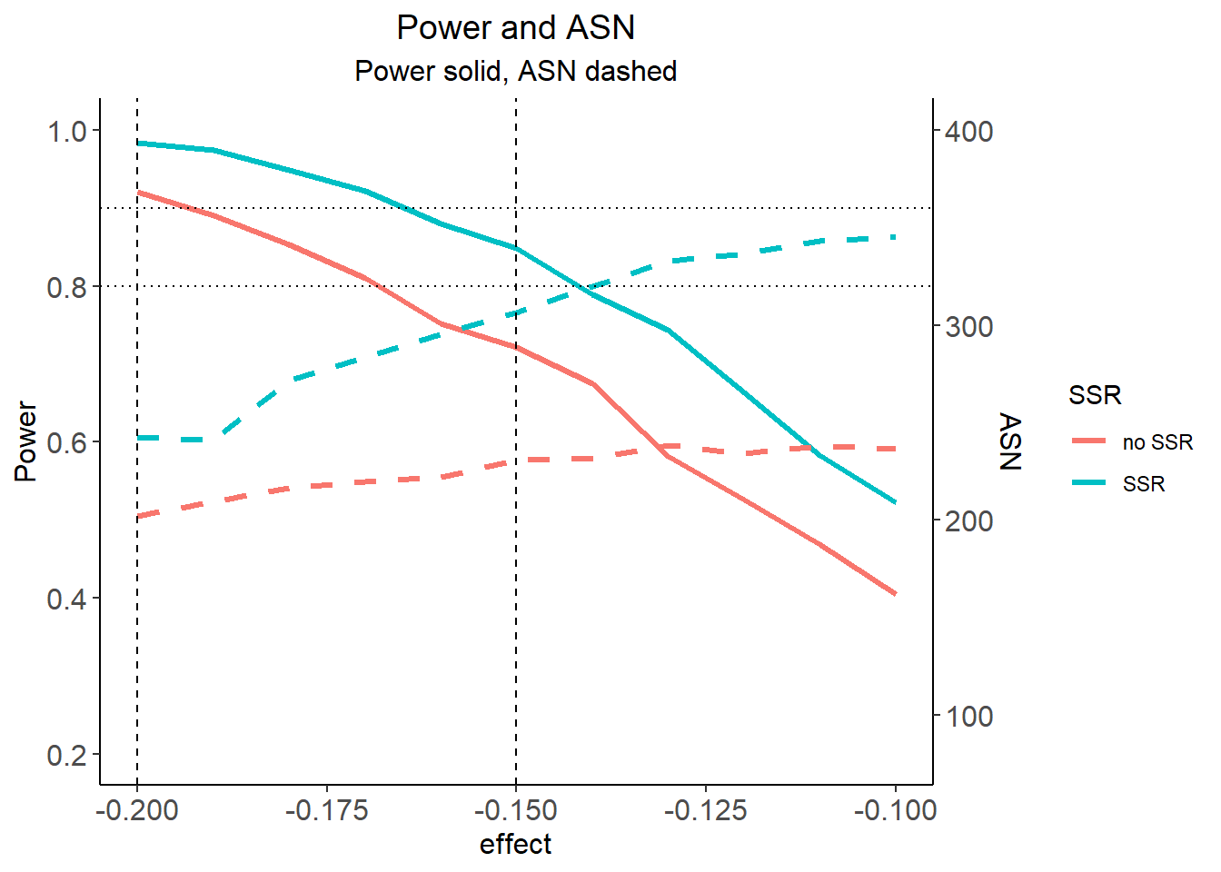
Exercise 4b (illustrate power difference)
Illustrate the gain in power when using the adaptive sample size recalculation.
Solution
We use ggplot2 for doing this. First, a data set df is defined with the additional variable SSR. Using mytheme and the following ggplots commands, the difference in power and ASN of the two strategies is illustrated. It shows that at least for effect difference > 0.15 an overall power of more than around 85% can be achieved with the proposed sample size recalculation strategy.
Warning: Using `size` aesthetic for lines was deprecated in ggplot2 3.4.0.
ℹ Please use `linewidth` instead.
plot(p)
# Note: for saving the plot, you could e.g. use the commented code below# ggplot2::ggsave(filename = "C:/yourdirectory/comparison.png",# plot = ggplot2::last_plot(), device = NULL, path = NULL,# scale = 1.2, width = 20, height = 12, units = "cm", dpi = 600, limitsize = TRUE)
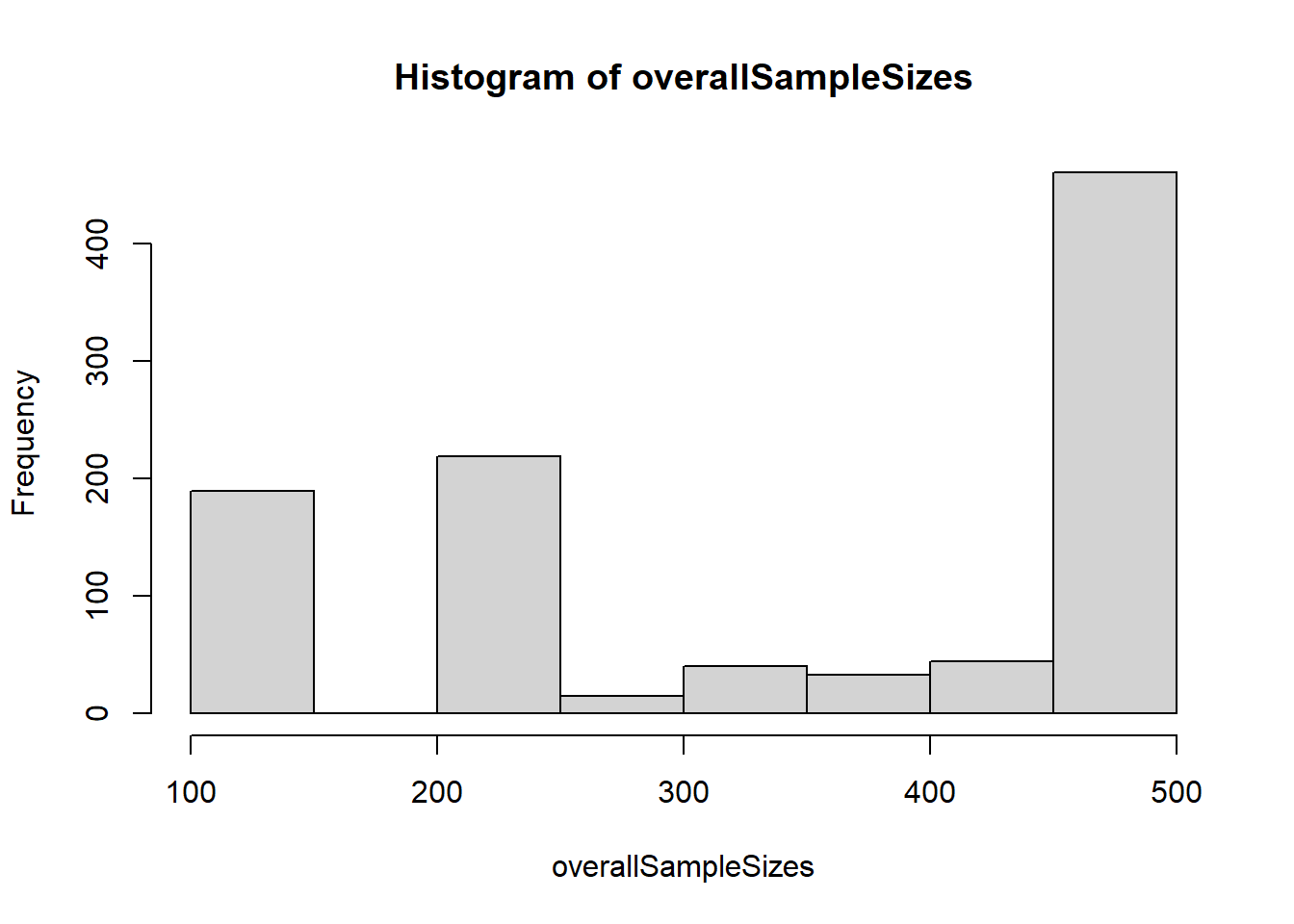
Exercise 4c (histogram of sample sizes)
Create a histogram for the attained sample size of the study when using the adaptive sample size recalculation. How often will the maximum sample size be achieved?
Solution
With the getData command the simulation results are obtained. Depending on pi1, you can create the histogram of the simulated total sample size
# tic()# overallSampleSizes <- numeric(maxiter)# for (i in 1:maxiter) overallSampleSizes[i] <- sum(simPart[simPart$iterationNumber==i,]$numberOfSubjects)# toc()hist(overallSampleSizes)
How often the maximum sample size is reached can be obtained as follows:
Exercise 5 (Multi-armed design with continuous endpoint)
Suppose a trial is conducted with three active treatment arms (+ one control arm). An adaptive design using the equally weighted inverse normal method with two interim analyses using O’Brien & Fleming boundaries is chosen where in both interim analyses a selection of treatment arms is foreseen (overall \(\alpha = 0.025\) one-sided). It is decided to test the intersection tests in the closed system of hypotheses with Dunnett’s test. In the designing stage, it was decided to conduct the study with 20 patients per treatment arm and stage where at interim the sample size can be redefined.
Exercise 5a (First stage and conditional power)
Suppose, at the first stage, the following results were obtained:
arm
n
mean
std
1
19
3.11
1.77
2
22
3.87
1.23
3
23
4.12
1.64
control
21
3.02
1.72
Perform the closed test and assess the conditional power in order to decide which treatment arm(s) should be selected and if the sample size should be redefined.
Multi-arm analysis results for a continuous endpoint (3 active arms vs. control)
Sequential analysis with 3 looks (inverse normal combination test design), one-sided overall significance level 2.5%. The results were calculated using a multi-arm t-test, Dunnett intersection test, overall pooled variances option. H0: mu(i) - mu(control) = 0 against H1: mu(i) - mu(control) > 0. The conditional power calculation with planned sample size is based on overall effect: thetaH1(1) = 0.09, thetaH1(2) = 0.85, thetaH1(3) = 1.1 and overall standard deviation: sd(1) = 1.74, sd(2) = 1.49, sd(3) = 1.68.
Stage
1
2
3
Fixed weight
0.577
0.577
0.577
Cumulative alpha spent
0.0003
0.0072
0.0250
Stage levels (one-sided)
0.0003
0.0071
0.0225
Efficacy boundary (z-value scale)
3.471
2.454
2.004
Cumulative effect size (1)
0.090
Cumulative effect size (2)
0.850
Cumulative effect size (3)
1.100
Cumulative (pooled) standard deviation
1.597
Stage-wise test statistic (1)
0.178
Stage-wise test statistic (2)
1.745
Stage-wise test statistic (3)
2.283
Stage-wise p-value (1)
0.4296
Stage-wise p-value (2)
0.0424
Stage-wise p-value (3)
0.0125
Adjusted stage-wise p-value (1, 2, 3)
0.0325
Adjusted stage-wise p-value (1, 2)
0.0751
Adjusted stage-wise p-value (1, 3)
0.0232
Adjusted stage-wise p-value (2, 3)
0.0231
Adjusted stage-wise p-value (1)
0.4296
Adjusted stage-wise p-value (2)
0.0424
Adjusted stage-wise p-value (3)
0.0125
Overall adjusted test statistic (1, 2, 3)
1.845
Overall adjusted test statistic (1, 2)
1.439
Overall adjusted test statistic (1, 3)
1.991
Overall adjusted test statistic (2, 3)
1.994
Overall adjusted test statistic (1)
0.177
Overall adjusted test statistic (2)
1.724
Overall adjusted test statistic (3)
2.240
Test action: reject (1)
FALSE
Test action: reject (2)
FALSE
Test action: reject (3)
FALSE
Conditional rejection probability (1)
0.0101
Conditional rejection probability (2)
0.0831
Conditional rejection probability (3)
0.1432
Planned sample size
40
40
Conditional power (1)
0.0009
0.0182
Conditional power (2)
0.4102
0.8723
Conditional power (3)
0.6722
0.9652
95% repeated confidence interval (1)
[-1.897; ]
95% repeated confidence interval (2)
[-1.065; 2.765]
95% repeated confidence interval (3)
[-0.794; ]
Repeated p-value (1)
>0.5
Repeated p-value (2)
0.2633
Repeated p-value (3)
0.1794
Legend:
(i): results of treatment arm i vs. control arm
(i, j, …): comparison of treatment arms ‘i, j, …’ vs. control arm
Exercise 5b (Second stage)
Suppose it was decided to drop treatment arm 1 for stage 2 and leave the sample size for the remaining arms unchanged. For the second stage, the following results were obtained:
arm
n
mean
std
2
23
3.66
1.11
3
19
3.98
1.21
control
22
2.99
1.82
Perform the closed test and discuss whether or not to stop the study and determine overall \(p\,\)-values and confidence intervals.
Multi-arm analysis results for a continuous endpoint (3 active arms vs. control)
Sequential analysis with 3 looks (inverse normal combination test design), one-sided overall significance level 2.5%. The results were calculated using a multi-arm t-test, Dunnett intersection test, overall pooled variances option. H0: mu(i) - mu(control) = 0 against H1: mu(i) - mu(control) > 0.
Stage
1
2
3
Fixed weight
0.577
0.577
0.577
Cumulative alpha spent
0.0003
0.0072
0.0250
Stage levels (one-sided)
0.0003
0.0071
0.0225
Efficacy boundary (z-value scale)
3.471
2.454
2.004
Cumulative effect size (1)
0.090
Cumulative effect size (2)
0.850
0.758
Cumulative effect size (3)
1.100
1.052
Cumulative (pooled) standard deviation
1.597
1.468
Stage-wise test statistic (1)
0.178
Stage-wise test statistic (2)
1.745
1.582
Stage-wise test statistic (3)
2.283
2.226
Stage-wise p-value (1)
0.4296
Stage-wise p-value (2)
0.0424
0.0594
Stage-wise p-value (3)
0.0125
0.0149
Adjusted stage-wise p-value (1, 2, 3)
0.0325
0.0274
Adjusted stage-wise p-value (1, 2)
0.0751
0.0594
Adjusted stage-wise p-value (1, 3)
0.0232
0.0149
Adjusted stage-wise p-value (2, 3)
0.0231
0.0274
Adjusted stage-wise p-value (1)
0.4296
Adjusted stage-wise p-value (2)
0.0424
0.0594
Adjusted stage-wise p-value (3)
0.0125
0.0149
Overall adjusted test statistic (1, 2, 3)
1.845
2.662
Overall adjusted test statistic (1, 2)
1.439
2.121
Overall adjusted test statistic (1, 3)
1.991
2.945
Overall adjusted test statistic (2, 3)
1.994
2.767
Overall adjusted test statistic (1)
0.177
Overall adjusted test statistic (2)
1.724
2.322
Overall adjusted test statistic (3)
2.240
3.121
Test action: reject (1)
FALSE
FALSE
Test action: reject (2)
FALSE
FALSE
Test action: reject (3)
FALSE
TRUE
Conditional rejection probability (1)
0.0101
Conditional rejection probability (2)
0.0831
0.3184
Conditional rejection probability (3)
0.1432
0.6154
95% repeated confidence interval (1)
[-1.897; ]
95% repeated confidence interval (2)
[-1.065; 2.765]
[-0.203; 1.716]
95% repeated confidence interval (3)
[-0.794; ]
[0.066; 2.022]
Repeated p-value (1)
>0.5
Repeated p-value (2)
0.2633
0.0476
Repeated p-value (3)
0.1794
0.0162
Legend:
(i): results of treatment arm i vs. control arm
(i, j, …): comparison of treatment arms ‘i, j, …’ vs. control arm
Exercise 5c (Intersection tests)
Would the Bonferroni and the Simes test intersection tests provide the same results?
Multi-arm analysis results for a continuous endpoint (3 active arms vs. control)
Sequential analysis with 3 looks (inverse normal combination test design), one-sided overall significance level 2.5%. The results were calculated using a multi-arm t-test, Bonferroni intersection test, overall pooled variances option. H0: mu(i) - mu(control) = 0 against H1: mu(i) - mu(control) > 0.
Stage
1
2
3
Fixed weight
0.577
0.577
0.577
Cumulative alpha spent
0.0003
0.0072
0.0250
Stage levels (one-sided)
0.0003
0.0071
0.0225
Efficacy boundary (z-value scale)
3.471
2.454
2.004
Cumulative effect size (1)
0.090
Cumulative effect size (2)
0.850
0.758
Cumulative effect size (3)
1.100
1.052
Cumulative (pooled) standard deviation
1.597
1.468
Stage-wise test statistic (1)
0.178
Stage-wise test statistic (2)
1.745
1.582
Stage-wise test statistic (3)
2.283
2.226
Stage-wise p-value (1)
0.4296
Stage-wise p-value (2)
0.0424
0.0594
Stage-wise p-value (3)
0.0125
0.0149
Adjusted stage-wise p-value (1, 2, 3)
0.0376
0.0297
Adjusted stage-wise p-value (1, 2)
0.0848
0.0594
Adjusted stage-wise p-value (1, 3)
0.0251
0.0149
Adjusted stage-wise p-value (2, 3)
0.0251
0.0297
Adjusted stage-wise p-value (1)
0.4296
Adjusted stage-wise p-value (2)
0.0424
0.0594
Adjusted stage-wise p-value (3)
0.0125
0.0149
Overall adjusted test statistic (1, 2, 3)
1.779
2.591
Overall adjusted test statistic (1, 2)
1.374
2.074
Overall adjusted test statistic (1, 3)
1.959
2.922
Overall adjusted test statistic (2, 3)
1.959
2.718
Overall adjusted test statistic (1)
0.177
Overall adjusted test statistic (2)
1.724
2.322
Overall adjusted test statistic (3)
2.240
3.121
Test action: reject (1)
FALSE
FALSE
Test action: reject (2)
FALSE
FALSE
Test action: reject (3)
FALSE
TRUE
Conditional rejection probability (1)
0.0101
Conditional rejection probability (2)
0.0756
0.2954
Conditional rejection probability (3)
0.1317
0.5764
95% repeated confidence interval (1)
[-1.901; 2.081]
95% repeated confidence interval (2)
[-1.068; 2.768]
[-0.227; 1.747]
95% repeated confidence interval (3)
[-0.798; 2.998]
[0.041; 2.051]
Repeated p-value (1)
>0.5
Repeated p-value (2)
0.2789
0.0518
Repeated p-value (3)
0.1915
0.0189
Legend:
(i): results of treatment arm i vs. control arm
(i, j, …): comparison of treatment arms ‘i, j, …’ vs. control arm
Multi-arm analysis results for a continuous endpoint (3 active arms vs. control)
Sequential analysis with 3 looks (inverse normal combination test design), one-sided overall significance level 2.5%. The results were calculated using a multi-arm t-test, Simes intersection test, overall pooled variances option. H0: mu(i) - mu(control) = 0 against H1: mu(i) - mu(control) > 0.
Stage
1
2
3
Fixed weight
0.577
0.577
0.577
Cumulative alpha spent
0.0003
0.0072
0.0250
Stage levels (one-sided)
0.0003
0.0071
0.0225
Efficacy boundary (z-value scale)
3.471
2.454
2.004
Cumulative effect size (1)
0.090
Cumulative effect size (2)
0.850
0.758
Cumulative effect size (3)
1.100
1.052
Cumulative (pooled) standard deviation
1.597
1.468
Stage-wise test statistic (1)
0.178
Stage-wise test statistic (2)
1.745
1.582
Stage-wise test statistic (3)
2.283
2.226
Stage-wise p-value (1)
0.4296
Stage-wise p-value (2)
0.0424
0.0594
Stage-wise p-value (3)
0.0125
0.0149
Adjusted stage-wise p-value (1, 2, 3)
0.0376
0.0297
Adjusted stage-wise p-value (1, 2)
0.0848
0.0594
Adjusted stage-wise p-value (1, 3)
0.0251
0.0149
Adjusted stage-wise p-value (2, 3)
0.0251
0.0297
Adjusted stage-wise p-value (1)
0.4296
Adjusted stage-wise p-value (2)
0.0424
0.0594
Adjusted stage-wise p-value (3)
0.0125
0.0149
Overall adjusted test statistic (1, 2, 3)
1.779
2.591
Overall adjusted test statistic (1, 2)
1.374
2.074
Overall adjusted test statistic (1, 3)
1.959
2.922
Overall adjusted test statistic (2, 3)
1.959
2.718
Overall adjusted test statistic (1)
0.177
Overall adjusted test statistic (2)
1.724
2.322
Overall adjusted test statistic (3)
2.240
3.121
Test action: reject (1)
FALSE
FALSE
Test action: reject (2)
FALSE
FALSE
Test action: reject (3)
FALSE
TRUE
Conditional rejection probability (1)
0.0101
Conditional rejection probability (2)
0.0756
0.2954
Conditional rejection probability (3)
0.1317
0.5764
95% repeated confidence interval (1)
[-1.901; 2.081]
95% repeated confidence interval (2)
[-1.068; 2.768]
[-0.227; 1.747]
95% repeated confidence interval (3)
[-0.798; 2.998]
[0.041; 2.051]
Repeated p-value (1)
>0.5
Repeated p-value (2)
0.2789
0.0518
Repeated p-value (3)
0.1915
0.0189
Legend:
(i): results of treatment arm i vs. control arm
(i, j, …): comparison of treatment arms ‘i, j, …’ vs. control arm
Bonus Exercise 6 (Planning of survival design)
A survival trial is planned to be performed with one interim stage and using an O’Brien & Fleming type \(\alpha\)-spending approach at \(\alpha = 0.025\). The interim is planned to be performed after half of the necessary events were observed. It is assumed that the median survival time is 18 months in the treatment group, and 12 months in the control. Assume that the drop-out rate is 5% after 1 year and the drop-out time is exponentially distributed.
Exercise 6a (accrual and follow-up time given)
The patients should be recruited within 12 months assuming uniform accrual. Assume an additional follow-up time of 12 months, i.e., the study should be conducted within 2 years. Calculate the necessary number of events and patients (total and per month) in order to reach power 90% with the assumed median survival times if the survival time is exponentially distributed. Under the postulated assumption, estimate interim and final analysis time.
Solution
In this simplest example, accrual and follow-up time needs to be specified. The effect size is defined in terms of lambda1 and lambda2 (you can also specify lambda2 and hazardRatio).
Sequential analysis with a maximum of 2 looks (group sequential design), one-sided overall significance level 2.5%, power 90%. The results were calculated for a two-sample logrank test, H0: hazard ratio = 1, H1: treatment lambda(1) = 0.039, control lambda(2) = 0.058, accrual time = 12, accrual intensity = 38.9, follow-up time = 12, dropout rate(1) = 0.05, dropout rate(2) = 0.05, dropout time = 12.
Stage
1
2
Planned information rate
50%
100%
Cumulative alpha spent
0.0015
0.0250
Stage levels (one-sided)
0.0015
0.0245
Efficacy boundary (z-value scale)
2.963
1.969
Efficacy boundary (t)
0.593
0.782
Cumulative power
0.2525
0.9000
Number of subjects
467.3
467.3
Expected number of subjects under H1
467.3
Cumulative number of events
128.3
256.5
Expected number of events under H1
224.1
Analysis time
13.14
24.00
Expected study duration under H1
21.26
Exit probability for efficacy (under H0)
0.0015
Exit probability for efficacy (under H1)
0.2525
Legend:
(t): treatment effect scale
ceiling(x1$maxNumberOfEvents)
[1] 257
ceiling(x1$maxNumberOfSubjects)
[1] 468
ceiling(x1$maxNumberOfSubjects)/12
[1] 39
x1$analysisTime
         [,1]
[1,] 13.14114
[2,] 24.00000
Exercise 6b (follow-up time and absolue intensity given)
Assume that 25 patients can be recruited each month and that there is uniform accrual. Estimate the necessary accrual time if the planned follow-up time remains unchanged.
Solution
Here the end of accrual and the number of patients is calculated at given follow-up time and absolute accrual intensity:
Exercise 6c (accrual time and max number of patients given)
Assume that accrual stops after 16 months with 25 patients per month, i.e., after 400 patients were recruited. What is the estimated necessary follow-up time?
Solution
At given accrual time and number of patients, the follow-up time is calculated:
How do the results change if in the first 3 months 15 patients, in the second 3 months 20 patients, and after 6 months 25 patients per month can be accrued?
Solution
This is the result from b), where the end of accrual is calculated:
Assume that the study from Example 6 is planned with 257 events and 400 patients under the assumptions that accrual stops after 16 months with 25 patients per month. Verify by simulation the correctness of the results obtained by the analytical formulae.
Solution
We first calculate the analysis times by the analytical formulas and verify that the power is indeed exceeding 90%:
Assume now that a sample size increase up to a ten-fold of the originally planned number of events is foreseen. Conditional power 90% based on the observed hazard ratios is used to increase the number of events. Assess by simulation the magnitude of power increase when using the appropriate method.
Simulate the Type I error rate when using
the group sequential method
the inverse normal method
Hint: Make sure that enough subjects are used in the simulation (set maxNumberOfSubjects = 3000 and no drop-outs)
Solution
First define an inverse normal design with the same parameters as the original group sequential design:
dIN <-getDesignGroupSequential(kMax =2, typeOfDesign ="asOF", beta =0.1)
The following simulation compares the Type I error rate of the inverse normal method with the type I error rate of the (illegal) use of the group-sequential method: